In a previous post we covered a quick and dirty introduction to deep Q learning. This covered the conceptual basics: an agent uses a deep neural network to approximate the value of its action-value function, and attempts to maximize its score over time using an off-policy learning strategy. The high level intuition is sufficient to know what’s going on, but now it’s time to dive into the details to actually code up the deep Q network.
In this post, we’re going to go over the deep Q learning algorithm and get started coding our own agent to learn the Atari classic, Space Invaders. Of course, we’re going to be using the OpenAI gym implementation of the environment, so don’t worry, we don’t have to reinvent the wheel.
To understand how deep Q learning works, let’s take a step back and evaluate the architecture for the “shallow” implementation of Q learning.
In traditional Q learning, the agent maps its current state and all possible actions onto a table that outputs the values of those combinations. Selecting the action with the largest value, for a given state, is greedy, and any other selection is exploratory.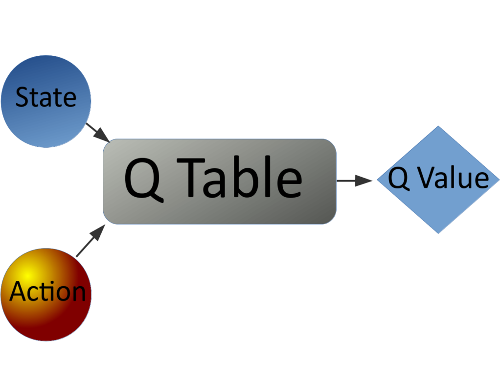 As we stated previously, Q learning is off-policy, so many of these actions will be exploratory, and the results of taking those actions will be used to update the Q table for the state action pair, according to the following equation:
$Q(S_{t+1}, A_{t+1}) = Q(S_{t}, A_{t}) + \alpha ( R_{t+1} + \gamma \underset {a} {max} Q(S_{t+1}, a) – Q(S_{t}, A_{t}))$
Where $ \alpha $ is the agent’s learning rate, and $ \gamma $ is the agent’s discount factor. Both are hyperparameters of the agent, and control the step size in updating the agent’s estimate of a state-value pair, and the extent to which the agent discounts future rewards, respectively. $ \alpha $ is typically chosen to be $ 0 \leq \alpha \leq 1 \simeq 0.1 $ and $ \gamma $ is usually chosen to be $ 0 \leq \gamma \leq 1 \simeq 0.9$
Q learning is a part of the temporal difference learning algorithms, which are both bootstrapped and model free. Bootstrapped means that the agent uses estimates of one state to update its estimate of other states, which is evidenced the presence of the $S_t$ and $S_{t+1}$ terms in the update equation for Q. The agent is effectively using the values of successor states to calculate the value of the previous states. They are model free in the sense that the agent does not need any prior information about the environment. It doesn’t need to know how one state transitions into another, how the rewards are distributed, or the rules of the game. All this information is discovered interacting with the environment. Best of all, this learning is done at each time step, hence the name “temporal difference”.
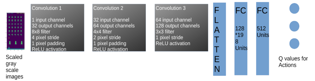
As we discussed in the last post, we run into problems when the state-action spaces become sufficiently large, or worse – continuous, so that the tabular representation of the Q function becomes impossible. In these cases, we have to transition to using a neural network to approximate the value of a state and action pair. This modification results in the following network architecture for deep Q learning:
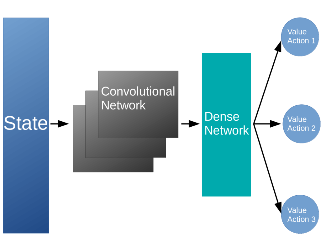
The state, typically the image of the screen, is fed into the convolutional neural network which reduces it to a more manageable subspace. This is passed into a dense network that is used to compute the values of each of the actions, given the current state. The agent can then use an $\epsilon$-greedy strategy to pick the next action, receive its reward, and perform the update to the Q network using back propagation.
The precise architecture of the convolutional neural network is typically problem dependent, and we will be using one that is different from the original implementation the deep mind team. The reason is that the input images are of different sizes, and we won’t be cutting down to an 84×84 pixel image. The screen image from space invaders in the OpenAI gym is initially 210×160 pixels, with 3 channels. The agent cannot move all the way to the left or right of the screen, so we can chop off some pixels on the left and right. Similarly, the ground isn’t involved in the action, so we can crop it out. There is some potential for this to go wrong, as cropping the left and right sides can obscure the aliens, however the agent can’t fire at them anyway so for a first pass at the problem, I’d argue the efficiency trade off is worth it. We also don’t need all the colors, since the colors don’t affect the game play, so we can gain further efficiency converting to a gray scale (but of course matplotlib converts it to a purple/green, whatever).
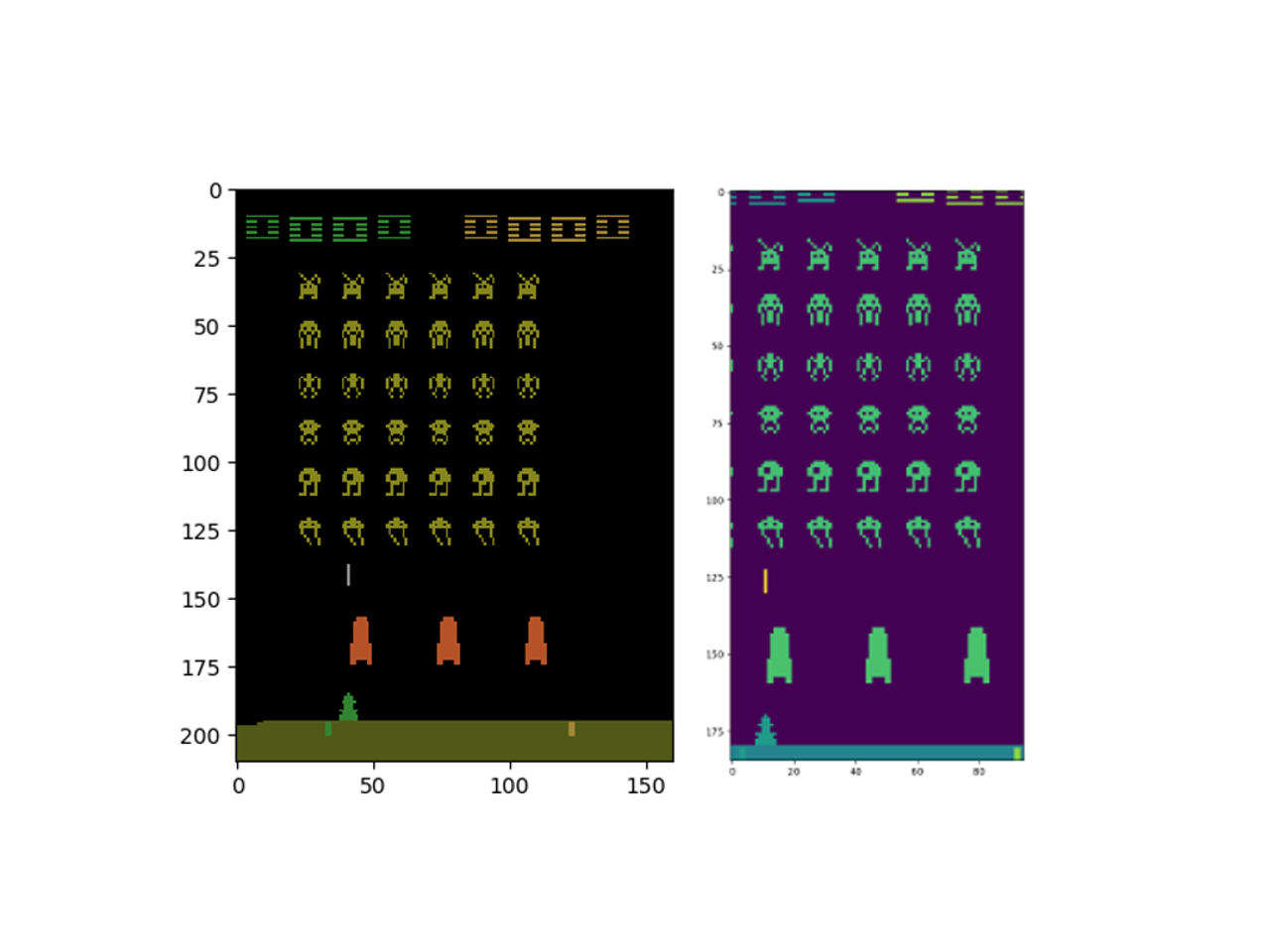
To achieve this, we’re going to slice the observation array: $observation[15:200,30:125]$ and take the mean, to get the gray scale: $np.mean(observation[15:200,30:125])$. This will be fed into the following neural network.
If you’ve been paying attention, you may have an objection. The point of this whole exercise is to get the agent to play the game. How the hell can it learn to play the game just seeing a single image at a time? The agent will have no idea which way the aliens are moving, for one problem. To deal with this, we have a simple solution. Instead of passing in a single image to the neural network, we’re going to pass in a series of them. In our case, we’ll use 3 images as our input to the convolutional neural network, as this is sufficient for the agent to get a sense of motion. Of course, more sophisticated solutions would rely on recurrent neural networks to process the sequence of images, but we can get surprisingly good results with just a few still images through our network.
Next question to address is: how does the agent learn from its experience? The first thing we need is a type of memory. The agent needs to know the state at time t, the state at time t + 1, the action it took at time t, and the reward it received at time t + 1. Remember the states are the observation arrays passed back from the Open AI gym environment, which we will be cropping and gray scaling. The actions are just integers from 0 to 5, and the rewards are the score received at each step. The most efficient way to store these is as a list that we append to, and we can convert it to a numpy array when we do the actual learning. This memory should be initialized in some way, and in my approach I’ve chosen to use actual game play. Set some maximum memory length, and play episodes using random actions until the memory is full.
To accommodate learning, we use the neat trick of experience replay. The agent will sample some batch of memories at random, feed forward this batch of states and use the Q values for these states to update its estimates. The network calculates the predicted value of the current state, $Q_{pred}$, for all actions, as well as the value for the maximum action, $Q_{target}$. These values are fed into the update equation for the weights. The weights are updated to minimize the mean squared error between $Q_{pred}$ and $Q_{target}$ using back propagation.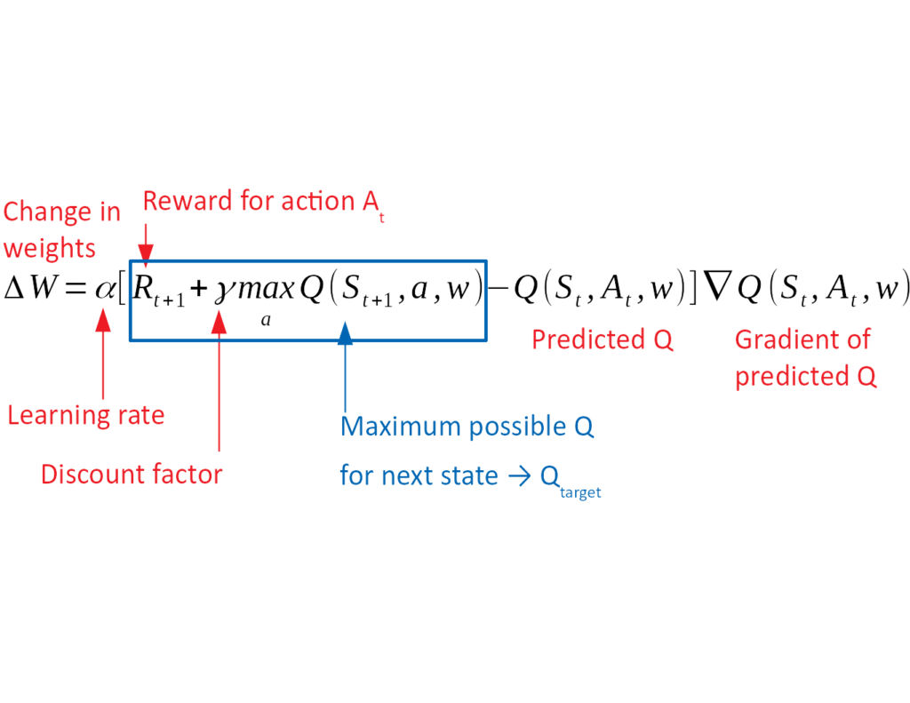
The final piece of this puzzle is how the agent converges on the greedy strategy. During the learn function we should include some functionality for reducing the $\epsilon$ over time, such that the agent settles on exploiting the best known action. Given the enormity of the parameter space, we don’t want to do this too quickly; the agent should have sufficient time to explore a meaningful portion of parameter space.
I’m making a Deep-Q Lunar Lander. Your tutorials, whether in text or video, are really valuable. Reading the original deepmind paper was theoretically great, but your explanation is taking me to a finished neural network today.
I did not understand the 128*19*8 on the first FC layer.
From were the 19 and the 8 came from?
Hey Renato, the 29*18 comes from the number of features that we get after taking all the convolutions.
So there are 128 filters, and each filter has 19*8 “pixels”.
I found this out the easy way, just printing out the dimensions of each layer after I did the feed forward operation. Hope that helps!
Most brief and precise tutorial!
I want to ask 2 question:
1. Which one is best for RL: Tensorflow, Pytorch or Keras?
2. Do you consider writing a book about Reinforcement Learning with Pytorch?
Sincerely.
I find pytorch to be the fastest and easiest to use, but that could just be me.
I haven’t considered a book as I prefer video content.
Hi Phil,
thanks so much for your videos! In your implementation
https://github.com/philtabor/Youtube-Code-Repository/blob/master/ReinforcementLearning/DeepQLearning/torch_deep_q_model.py#L92
, the loss function takes the parameters Qtarget and Qpred. However, due to the way that python variable bindings work, aren’t those two the same object?
Relevant code with comments to illustrate what i mean:
Qtarget = Qpred # this binds the object in Qpred to the variable name Qtarget
indices = np.arange(batch_size)
Qtarget[indices,maxA] = rewards + self.GAMMA*T.max(Qnext[1]) # doesn’t this change Qpred as well, because both variables refer to the same object
analogous example to show the same effect:
a = [1,2,3]
b = a
b[1] = 9000
# a is now [1, 9000, 3]
b is a # evaluates to True
Regards,
noh3
Yes, you are correct. It’s a typo. It should be Qtarget = Qpred.clone()
I have fixed this in the github as of now. Good spot!
Cool, thanks again! 🙂